Machine Learning Part 3: Ranking

April 4, 2013 by

Victor Marak

INTRODUCTION: In the previous article, we saw the utility of Naïve Bayes Rule for malware classification. While simple to understand and implement, we have tried to illustrate the best of its use writing our own Android malware classifier. The limitations of Bayes rule largely relates to the development of rules around a dataset, the quality of the dataset, and the optimum handling of outliers. Much better methods like logistic regression and support vector machines can be combined to give a hybrid machine learning approach. However, the goal of this article is to further explore the use of Bayes Rule and incorporate another technique of ranking. We will see how we might process an email corpus and segregate the mails from spam as well as understand the concepts in the process.

Learn Cybersecurity Data Science

Build your skills using machine learning and other cutting-edge tools to perform various cybersecurity tasks.

Start Learning

Limitations of Bayes Rule

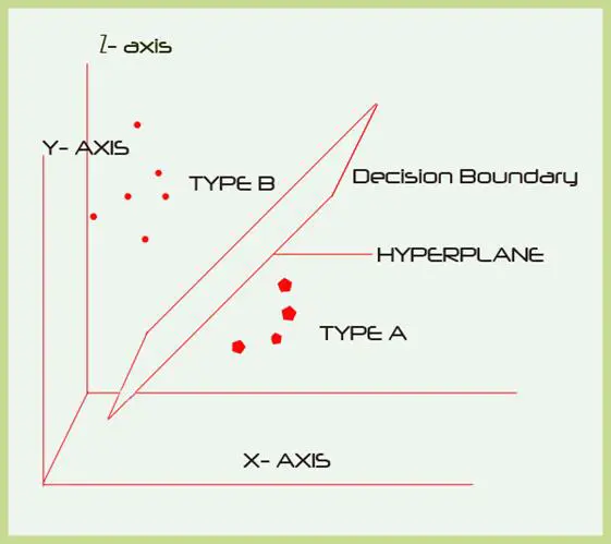
"Decision boundary" is a term that often comes up when trying to classify a dataset into two or more categories. Binary classification relates to being either this or that kind of an expected output. In many cases this is feasible. However in such cases, the number of features that are taken into account for making the final decision are limited. The term comes from graphing the variables to a two-dimensional plane wherein the classification can be visualized as a boundary – a single line that clearly demarcates the two classes. The classification can be embellished by taking into account other features as well. Doing this enables us to move beyond a simple probability product count and a comparison thereof between the numbers obtained from either class.

While taking into account the use of probability as floating point numbers, minuscule denormal numbers are not in the range of standard floating point types and is a side effect of continuous product of small floating point numbers. The solution to this problem can be applied using logarithms to represent a normalized range of such values. Logarithms can be thought of as a function that returns the power of and input corresponding to a base number: such as, if the function is given the input 1000 and the base number is set as 10, then the function would return the value 3, because 10^3 = 1000. This effectively means that large numbers such as 10000000 can be represented as 7 in a rescaled axis. This makes working with large quantities manageable. A thing to know from fundamental mathematical axioms is that any number raised to the power zero equals one. Therefore any number is fed as input and equals to 1, then the log will return the value 0. This could render an entire set of calculations to zero if products are implemented, which could be certainly the case when dealing with conditional probability. A simple technique used to alleviate the situation involves adding 1 to every output of the log value. This ensures that zero never occurs.

Natural logs are also a great way to work with a set of non scaled ranges as it uses e=2.713 as a base number. The value e occurs in many natural phenomena like the shape of a spiral, rate of decay of radiation and many other naturally occurrences. Thus making use of Ln makes a lot of sense in squashing the data to a suitable range.

Ranking

The process for ranking is akin to a threat modelling system rather than a vanilla classifier because it takes into account more features from the data set, in order to reach its conclusion--usually set as a final score. For building a combined feature set for the final score a set of individual features from the data set has to be composed which can include any number of features that can help in the final ranking process. Ranking is a lot like sorting, in that in the end if the ranking algorithm works, it automatically collates the respective items higher or lower in the list. For instance, in a malware rating system that is set up to give high priority to malware files, the benign files can be expected to float to the bottom of the ranked list out of a random sample set. That would be the best-case scenario, and in that case, the density function graphs can be plotted which is basically the count of items having a particular score and the threshold score for effective segregation can be empirically deduced.

An important procedure while working with a ranking system is the application of weights to a particular scoring data set. Weights are something that are also present in neural networks, however in this case the concept is the same while bearing a much more simplistic representation of the learning processes that occur in a neural net. Weights are simply numbers that are multiplied with a feature value that will influence the final score for that feature set. This process would make sense in practice as certain feature values have more importance/influence/occurrence on a particular sample set.

However this does not translate into a direct number input that would give a sure shot score every time. Once other features are included, the weighting numbers that are derived might have to be tuned to give the optimal balanced score for the cumulative feature set rank score. This is admittedly more of an art than a science as the black box effect of a working system after a certain set of weights are calibrated give it a magic effect of sorts. You won't know the exact mechanism but it might just perform very well.

Ranking takes a similar approach to score calculation in that –

1. A histogram is developed for a particular feature set. That is a vector is composed per item taking the individual features – like permissions of an AndroidAPKfile.
2. A frequency count is done on the vector set of the number of individual items having a particular feature (per column, per vector). This would give us the histogram data.
3. This histogram is sorted and the entire range, or a good portion thereof, is used to build the dataranking set.
4. Assuming that the histogram is done and that it reflects the statistical count of a particular feature component in the entire sampling corpus, the next step would be to take note of the individual values and reduce the differences in the count values especially if they are too large over the entire set, as this would give a very skewed score.
5. Taking the natural log (ln) of each of the values gives us a more flattened line when visualized in a graph. These values are the derived weights that will be used to give each feature in the data set a final value in the ranking system
6. Repeat this for every other feature set that is relevant to our ranking scheme. This will require choosing the feature sets carefully and may involve trial and error. Repeating this step will give us another set of vectors for each selected feature set. For illustrative purposes, this can be the API types most found in a particular sample set for Android malware and benign files.
7. The score is calculated by multiplying each weight of every feature found in the test set referring from the prior obtained data set, and then multiplying each of the final feature scores of every other feature. This would be the final score that will be used for ranking purposes.
8. Finally the list is sorted in descending order with the highest score on the top and the lowest at the bottom.

The benefit of this ranking procedure is evident in that it incorporates multiple feature sets towards the final ranking process –unlike using just the probability distribution data. The threshold score which can be used for classification has to be empirically assigned based on the scores obtained.

Spam Classification and Ranking

Spam mails can be represented as text files ignoring other data for now like attachments.

Each email has something called a header which is more like a manifest of the route that mail took to get from its source to its destination. For our purposes temporal or timeline based data will certainly be useful such as email send and receive times, the highest number of senders and their recipients etc. However this will be more of an exercise in brevity and as such will be kept simple to demonstrate the process, rather than build an enterprise level spam hitter – as much of the spam filtering has moved on to more complicated and effective mechanisms like matrix factoring (used in Netflix competition) and support vector machines (SVM).

Assuming a corpus consisting of spam mails and good mails, how do we start preparing the scoring data?

1. We could skip the headers for now.
2. Move on straight to the body and make a listing of the keywords in each mail. For this step, a vector has to be composed containing each term occurring in the mails (including redundant/repeating ones – important in fact). For this step each row will represent one email and the first column will be the email body text, represented in a single line.
3. Then a list of the English words is made that occur in the vector list. After this step a sorted list of the most occurring terms will be available. Take a histogram of the top ranking word counts and sort it. Being by taking a count of the total number of mails that have a particular English word in both the spam set and the good mail set. Make separate lists of the counts. Divide each of the top ranking term counts; say the top 20 or so with the total sample set counts from where the term frequencies are calculated. At this point we will have both the probability numbers and the counts themselves which will be used to derive the rank weights. At this point a simple Bayes' classifier can be coded using the values in the list just based on the text term frequencies. This exercise is similar to the Android file permissions Bayes classification exercise in the previous articles.
4. For the preceding steps a simple line reading function can be utilized that reads an email and saves the entire body text as a character array or an array of lines in a separate data structure that represents not only the body text lines but also other parameters for each email –like the timestamp and IP addresses.

   This data can be further used to blacklist emails using IP addresses and other header data. In addition, something more needs to be done with this data set that involves cleansing it for redundant English words. In anti-spam technology jargon these words are called stop words. Further numbers and punctuation have to be removed so that the remaining words themselves are cleanly represented. These strings related activities can be done in any programming language though specific languages like Perl have an obvious advantage towards linguistic processing.

5. Data set preparation and input range handling are the most important set of activities in any machine learning process and this comes up time and again. For our ranking scores we will both the spam and good mails training set as input without worrying about the type of mails for this score collation.

For our ranking purposes the sender's frequency list can also be calculated using a similar process. At the end of both these activities we get a histogram of the terms most occurring with reference to. both spam and genuine mails. We also have a histogram of the senders who are the most active.

Taking natural logs of both these features' values from each list individually gives us a set of calibrated weights.

Now run the same data extraction and processing algorithm on the test sets for both spam and good mails. Then, write a new function to calculate the total rank score of each email analysed.

Search for the email body text and for every term encountered multiply the weight associated with the term.

Similarly, multiply the sender's weight for every sender's id in the mail.

Multiply both these values to get the two feature ranking system.

Now sort these mails according to score.

This will give an effective demonstration of the final rank list. The mail ranks can now be checked for validity and tweaks can be made as well as incorporating more features from the manifest and other data from the mail like attachment size and type of files etc can add more depth to the ranking and classification process.

Conclusion

Learn Cybersecurity Data Science

Build your skills using machine learning and other cutting-edge tools to perform various cybersecurity tasks.

Start Learning

Data is becoming more complex and larger by the minute. How do we make sense of data around us and how can we use that obtained data for future prediction and categorization?These are well oiled inquiries that have kept statisticians and mathematicians busy for centuries giving rise to a body of knowledge to which we can refer and build upon. In this article, we have taken a better look at applying the similar steps towards implementing Bayes rule for classification purposes and embellished the process by using another technique of ranking. Both methods seem to work on the same data set while giving different uses to the obtained data to be better when leaning to work on new data. None of the above techniques are exact processes and might require several steps of data set filtering and values tweaking before the final results are optimal. In relation to newer and more advanced techniques, Bayes Rule has been quite effective for simple classification tasks. However, complex data sets that are not correlated linearly have to be analysed to give a better mathematical fit towards the pattern displayed by the data in question. In these cases Bayes rule can be safely abandoned keeping in mind the complexity to be dealt with when moving to more effective methods.